Factoring problem with quantum Fourier transform: an intuitive approach
One major application of quantum computing is cryptography. The commonly used encryption method RSA based on multiplying two large prime numbers \(N=xy\). In classical computing, there is no easy way to figure out the two prime numbers \(x,y\) given their product \(N\). With quantum computing, the decomposition can be found in polynomial time, much faster than existing classical computing algorithms.
The naive way to decompose is to try every possible number smaller than \(N\). But, we can propose a random guess \(x\), and there is an efficient algorithm to make the original naive guess into a much better guess \(x'\) that is very likely to be a factor of \(N\). We will explain first mathematically why can we convert a random guess into a better guess, and then how quantum computing can make this conversion process fast.
Why there is a better guess than a random number \(x\)
Let’s start with a random guess x, and most likely it is not a factor of N (otherwise problem solved!) The question is can we find certain function \(f(x)\), such that \(f(x)\) can be related to the factors of \(N\)? Surprisingly the answer is yes and the function is very simple: \(f(x) = x^p\).
Imaging we can find certain \(x^{p} \mod N = 1\) and if p is even, we have \[(x^{p/2}+1)(x^{p/2}-1) \mod N=0 \\ (x^{p/2}+1)(x^{p/2}-1)=mN\]
where m is an integer. Intuitively, the two factors must contain some information about factors \(x, y\). Mathematically, \(gcd(x-1,N), gcd(x+1,N)\) is a nontrivial factor. This way we successfully find a much better guess, which directly converts to the factorazation of N from some random guess with negligible connection with N.
Why quantum computing has an advantage to find the \(x'\)?
You may think this is simply a conversion of the factoring problem to another equivalent order-finding problem, which is also hard. Classically, we can still find the order \(p\) with classical computing resources, so why quantum computing has an advantage. To understand this, we need to realize that:
- order finding function is a periodic funciton, and periodicity is the solution \(p\).
- quantum computer is good at finding the periodicity via quantum Fourier transform
Let’s start with the first statement. We will see that how periodicity shows up in the modulus function.
1. Order finding function and its periodicity p
periodicity: \(x^m modN=x^{m+p}modN\)
Consider for certain value of p, \(p\)x^{p}modN=1\(. This is equivalent to\)x^{p}=k_pN+1$$.
For arbitrary integer m, if \(x^m modN = s\), or equivalently, \(x^m = k_m+s\), then for \(x^{m+p}\), we will have \[\begin{align*}x^{m+p}&=(k_mN+s)(k_pN+1)&=k_mk_pN^2+(k_m+k_p)N+s&=k_{m+p}+s \end{align*}\]
Therefore, \(x^{m+p}modN = s = x^m modN\), and the function \(x^m modN\) is a periodic function of m.
2. Quantum Fourier transform to find the periodicity p
Classically, to find the periodicity of certain function, Fourier transform is a handy tool to use. In practice, the periodicity in time/space domain can be visualized in frequency/spatial frequency domain. The Fourier transform is considered as a change of basis, and the basis can be visualized in the following discrete case:
Discrete Fourier transform
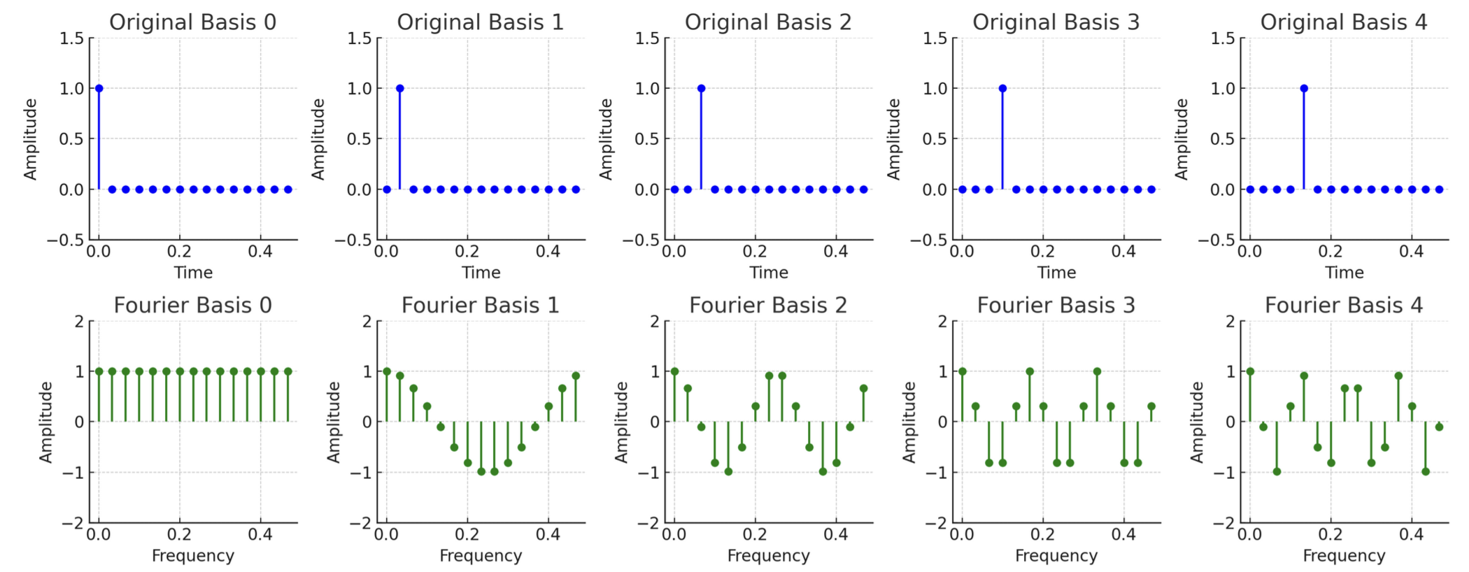
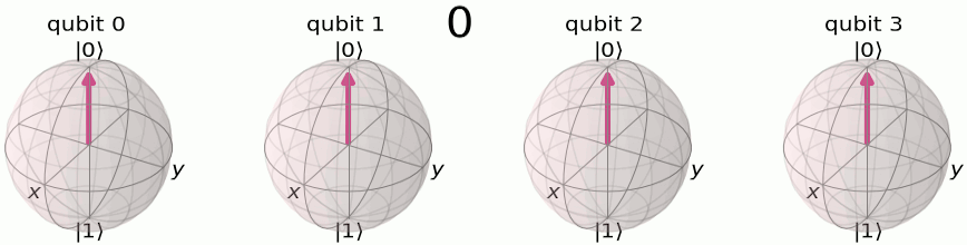
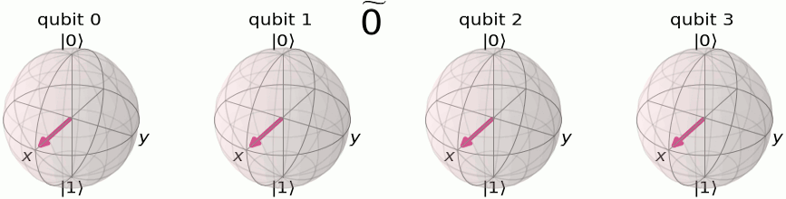
Quantum Fourier transform is also a way to represent the state in different basis. The difference that the original qubit basis is a two-dimensional complex space. Here, we first visualize the basis and we adopt a helpful notation: \(\ket{3}, \ket{\tilde{3}}\) to represent before and after Quantum Fourier transform, respectively. Here x, y can be represented in the binary format as \(\ket{x}=\ket{x_1x_2x_3...}\)
The QFT process of changing the basis from original to Fourier basis follows the derivation: \[\begin{align*} \text{QFT}\ket{x} &= \frac{1}{\sqrt{N}} \sum_{y=1}^{N}e^{2\pi ixy/N}\ket{y} \\ &= \frac{1}{\sqrt{N}} \sum_{y_1=0}^{1} \ldots \sum_{y_n=0}^{1} e^{2\pi ix\sum_{m=1}^{n}y_m 2^{n-m}/2^{n}}\ket{y_1\ldots y_n} \\ &= \frac{1}{\sqrt{N}} \sum_{y_1=0}^{1} \ldots \sum_{y_n=0}^{1}\prod_{m=1}^{n} e^{2\pi ixy_m/2^{m}}\ket{y_1\ldots y_n} \\ &= \frac{1}{\sqrt{N}} \sum_{y_1=0}^{1} \ldots \sum_{y_n=0}^{1} \otimes_{m=1}^n e^{2\pi ixy_m/2^{m}}\ket{y_m} \\ &= \frac{1}{\sqrt{N}} \left(\ket{0}+e^{2\pi ixy_1/2}\ket{1}\right)\left(\ket{0}+e^{2\pi ixy_2/2^{2}}\ket{1}\right)\ldots\left(\ket{0}+e^{2\pi ixy_n/2^n}\ket{1}\right) \end{align*}\]
Here we use the binary representation of \(j\) as \(j={j_1j_2j_3...j_n} =j_12^{n-1}+j_22^{n-2}+...+j_n\). The results of the derivation are visualized in the Bloch spheres representation of QFT basis . Intuitively, each qubit is rotated at a different phase speed corresponding to the binary representation, and the qubit with larger index m rotates slower, with a phase speed of 2pi/2^n while the first qubit is jumping with a phase speed 2pi*1/2, which basically jumps back and forth.
To find the periodicity of mod-function, we consider a unitary operator defined as calculate the mod of the multiplication: \[U\ket{x}=\ket{ax\mod N}\]
For a simple example \(x=3, N=5\), we have \(\ket{3},\ket{4},\ket{2},\ket{1}, \ket{3}...\)
The eigenstate of U can be defined as \(u_0=\ket{3}+\ket{4}+\ket{2}+\ket{1}\) as \(U\ket{u_0}=\ket{4}+\ket{2}+\ket{1}+\ket{3}\) due to the periodicity of the mod operation. More generally \[\begin{align*}\ket{u_{\phi}}&=e^{i\phi}\ket{3}+e^{i2\phi}\ket{4}+e^{i3\phi}\ket{2}+e^{i4\phi}\ket{1} \\U\ket{u_{\phi}}&=e^{i\phi}\ket{4}+e^{i2\phi}\ket{2}+e^{i3\phi}\ket{1}+e^{i4\phi}\ket{3}=e^{-i\phi}\ket{u_\phi}\end{align*}\]
Notice we need \(4\phi=2n\pi\), and we notice \(r=4\) is exactly the period or the order we are looking for and \(e^{i2\pi s/r}\). In general, the state is an eigenstate for any integer value of s, we have \[U\ket{u_{s}}=e^{-2\pi i s/r}\ket{u_s}\]
and the value r here would satisfy \(x^r \mod N = 1\). We will see that the periodicity r can be estimated via the quantum phase estimation by directly writing the phase into Fourier basis with a trick called phase kickback.
Phase kickback: use redundant qubits to extract the phase information.
\[CU(\frac{1}{\sqrt{2}}(\ket{0}+\ket{1})\ket{\psi})=\frac{1}{\sqrt{2}}(\ket{0}+e^{i\phi}\ket{1})\ket{\psi}\]It has an interesting consequence that after the control-gate operation, the state being controlled is not change, but the phase information is encoded into the controlling qubit. As if you push a button, nothing happened but you have yourself rotated by a (phase) angle.

(cartoon created by chatgpt)
This phase information can be extracted by applying a H-gate, which can be thought of a change of basis.
Following this idea, we can use multi-phase kickback trick to direct write the phase information into Fourier basis in its binary form! And after the inverse-quantum Fourier transform, the phase information can be retrieved and measured.
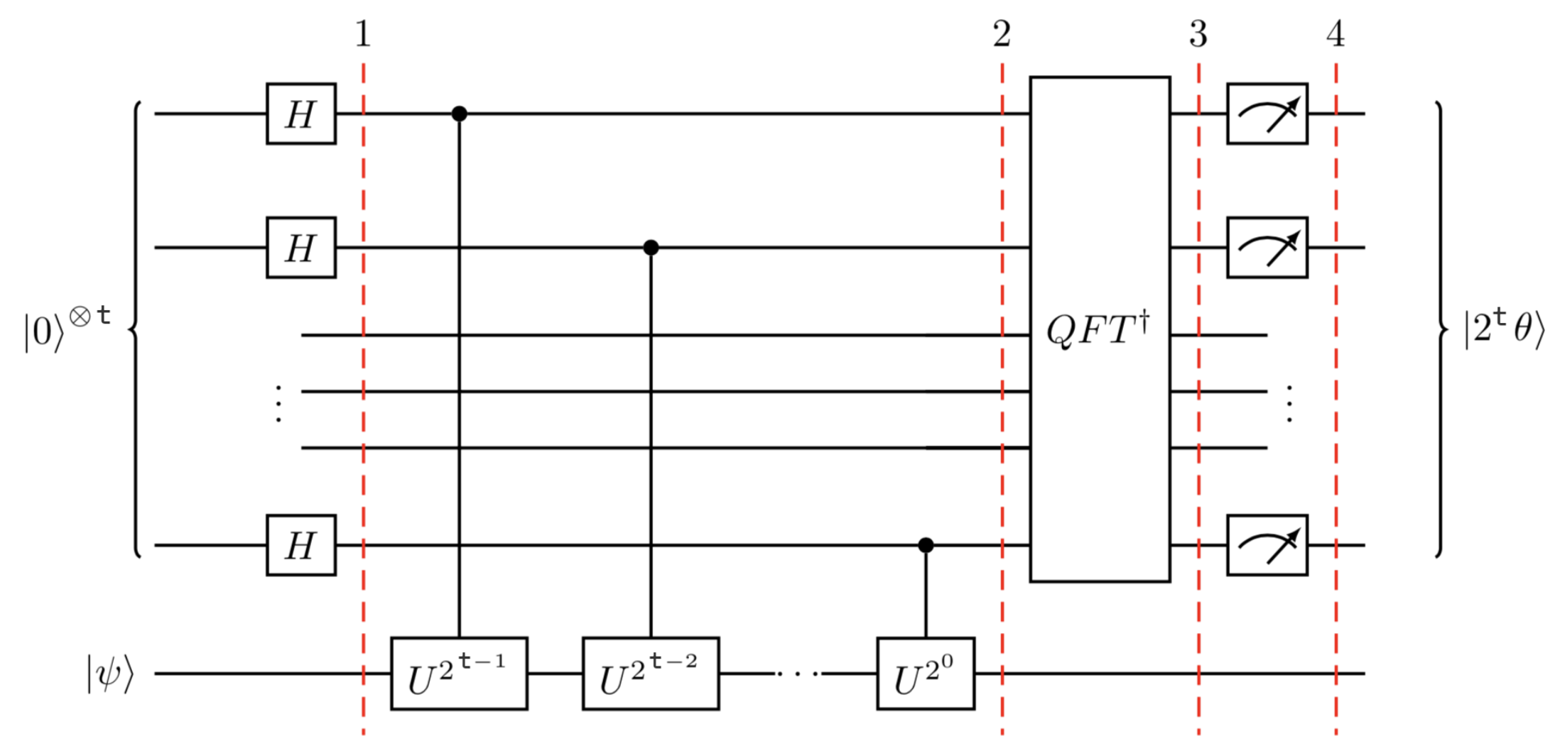
In conclusion, we start with a unitary operator for mapping to the mod of N. The multi-phase kickback trick allows us to directly write the phase of such unitary operator into the Fourier basis and get measured. The phase is actually the solution to the order-finding problem, which provides a better guess to the original quantum factoring problem.